1D Function Approximation Using a Neural Network
[Or how to create a neural network from scratch. This post was mainly inspired by Michael Nielsen's book on neural networks, and the 1989 paper by Cybenko. You can jump straight to the companion notebook if you like reading code more than tedious prose and awful jokes.]
Points and Functions
See these points?
| Random points on a grid, except they are not random. | |
|---|---|
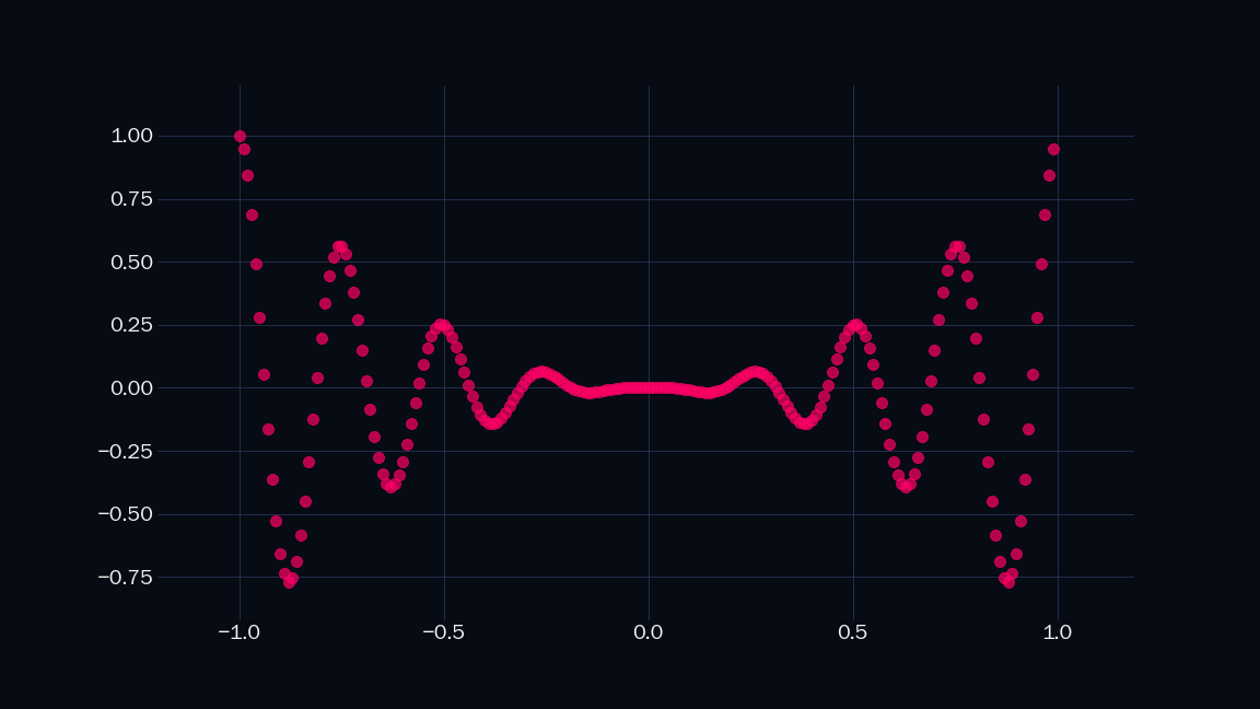 |
|
They are drawn from a function. Like $\sin(x)$. Or $\cos(x)$. Or $\frac{\zeta(\log(x^5 + 1))}{1 - \exp(1 - \sin(x^2) - \cos(x^2))}$. Let's call it $\mathsf{y(\mathit{x})}$. It is univariate, which means it takes a single real number $x$ as its input. I have plotted $\mathsf{y(\mathit{x})}$ for $200$ equispaced values of $x$ from $-1$ to $1$. Without knowing what $\mathsf{y(\mathit{x})}$ actually is, can we evaluate it for more values of $x$?
We can certainly guess values in between the red dots. We can manually paint in more dots, but this isn't a sustainable, scalable, or elegant solution to this problem. What if we had millions of such points, for billions of unknown functions?
| Function approximation by MS Paint. | |
|---|---|
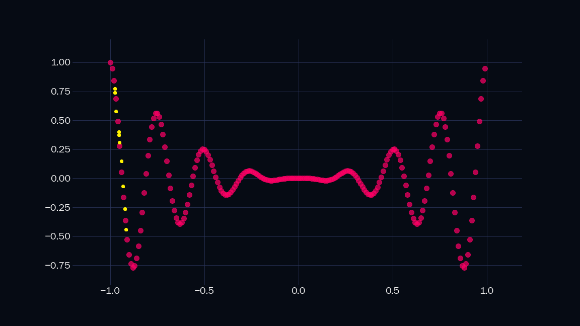 |
|
What if, instead of trying to guess what function these points come from, or manually drawing dots, we chose a type of function that can be shaped into any curve, by adjusting its parameters? We can then use it to approximate our unknown function, based on the points we have. For example, the function $\mathsf{f(\mathit{x}) = a \mathit{x} + b}$ is parametrized by $\mathsf{a}$, and $\mathsf{b}$, which need to be fixed before evaluating the function for any input $\mathit{x}$. Therefore, $\mathsf{a \mathit{x} + b}$ represents a family of functions, for different values of a, and b.
The Sigmoid
Here is what the sigmoid function looks like.
| $ \mathsf{ {\sigma} ({w \mathit{x} + b}) = \dfrac{1}{1 + e^{-(w \mathit{x} + b)}}}$ |
|---|
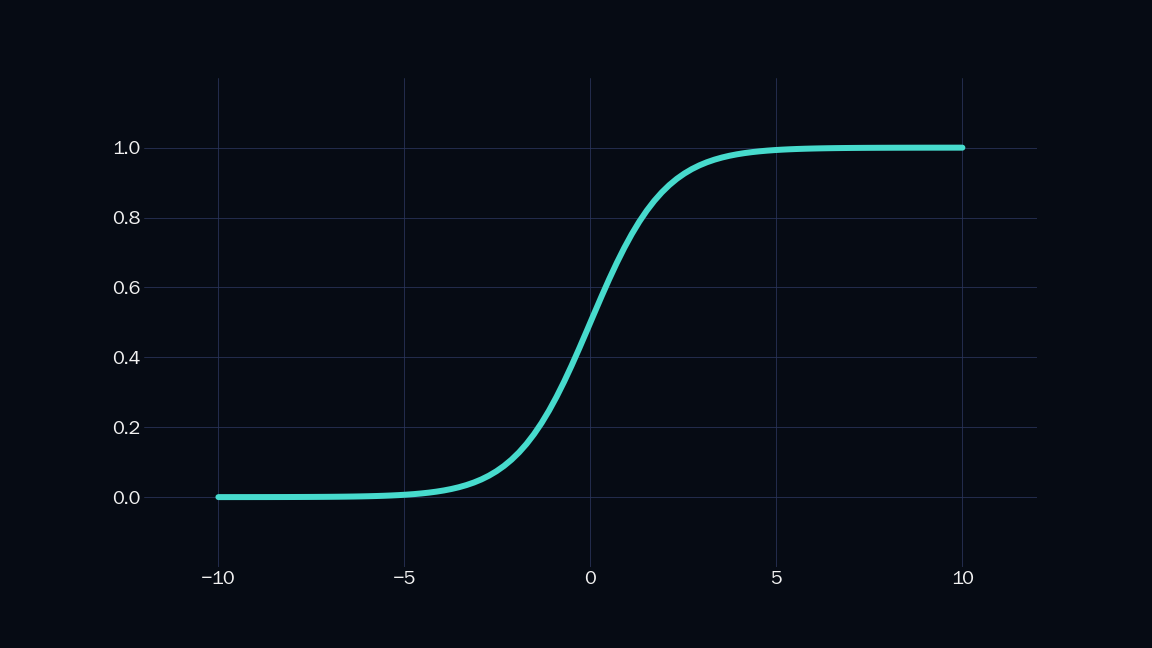 |
The sigmoid is parametrized by $\mathsf{w}$ and $\mathsf{b}$, which can be used to control the steepness and position of the sigmoid. We can combine two sigmoids to get a shape like this:
| $ \mathsf{ \dfrac{1}{1 + e^{-(60 \mathit{x} + 200)}} - \dfrac{1}{1 + e^{-(60 \mathit{x} + 20)}} }$ |
|---|
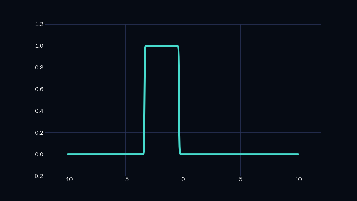 |
Let’s call the above shape an indicator. Note that it is just a sum of two sigmoids. It is $1$ in a specific range, and $0$ everywhere else in the number line. We can scale (i.e. mutiply by a constant) and add any number of such indicators to approximate any shape to arbitrary precision. Below is a demonstration, where $n$ is the number of indicators I have used.
| $n = 10$ | $n = 20$ |
|---|---|
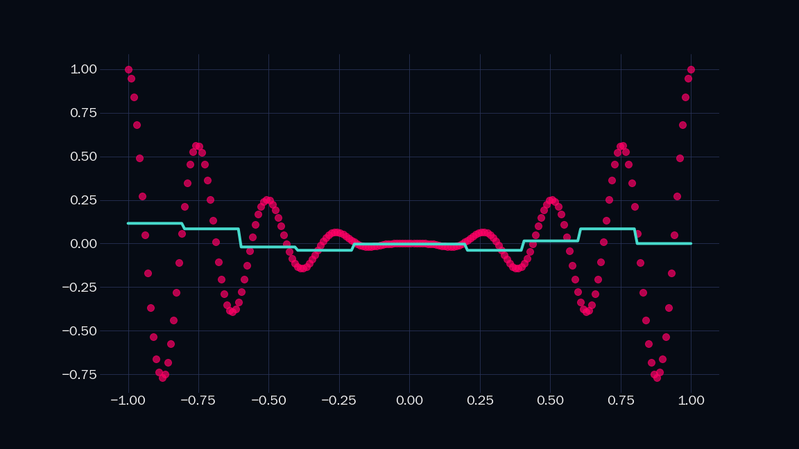 |
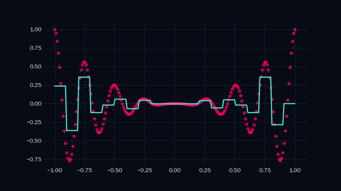 |
| $n = 30$ | $n = 40$ |
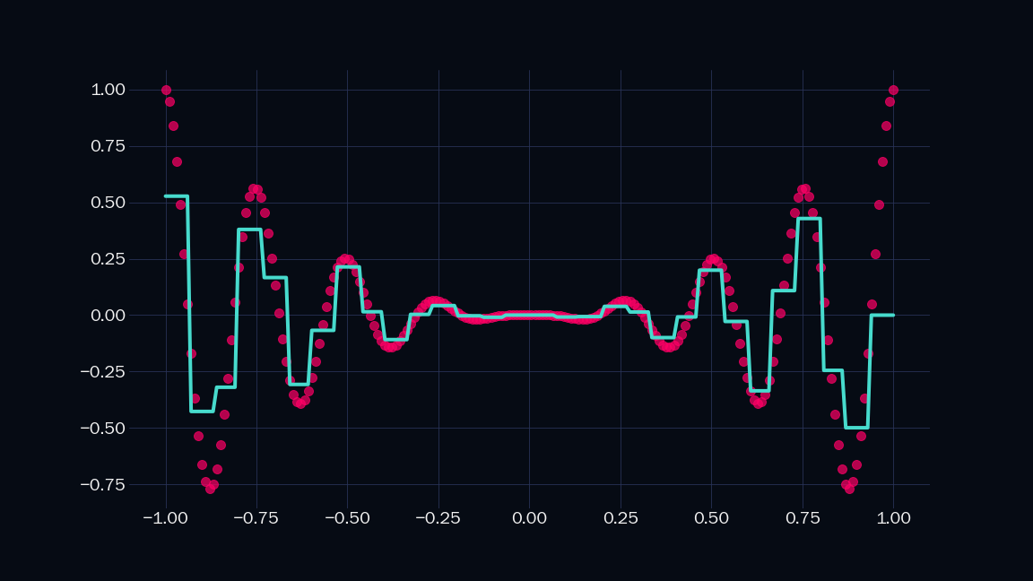 |
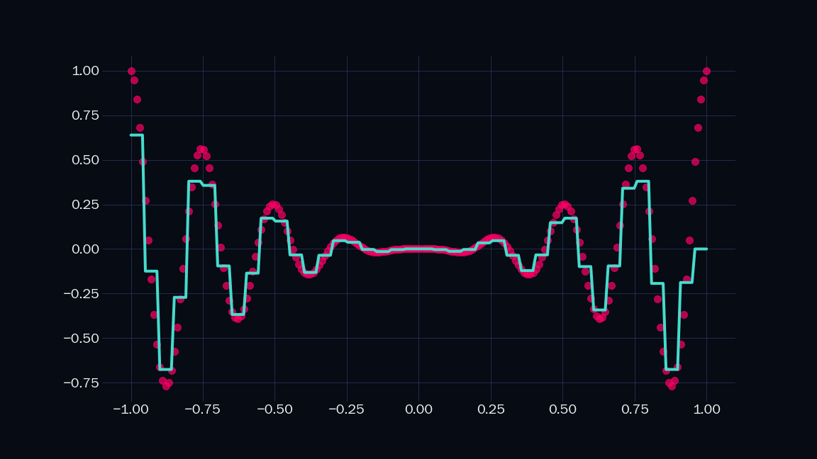 |
By increasing $n$ indefinitely, we can achieve arbitrary precision! But a few caveats:
- I did not use any sigmoids for the above plots, as that would have required me to find out the weights ($w$ and $b$) of all the sigmoids, and that involves more maths.
- The indicators above are simply the average of the target function in specific ranges (which become smaller as $n$ increases), and practically we cannot increase $n$ indefinitely in this method, because we have a limited sample of the target function.
- The point here was to provide a visual proof, that sigmoids can approximate any function, theoretically. How to do it actually?
A modest neural network
Let us frame everything we have discussed so far mathematically.
- Any target function can be approximated up to arbitrary precision by adding a bunch of indicators, each multiplied by a different constant.
- An indicator can be approximated by adding two sigmoids, each parametrized uniquely.
Therefore
- Any target function can be approximated by a sum of sigmoids, each multiplied by a constant, and parametrized uniquely. Or, to to put it simply:
| $\mathsf{ {f} ( {x} ) = { \displaystyle\sum\limits_{k = 1}^L} \color{white}{v_k} \sigma( \color{white}{w_k} {x} + \color{white}{b_k} ) }$ |
| The expression represents the summation of $\mathsf{L}$ sigmoids, each having parameters $\mathsf{w_k}$ and $\mathsf{b_k}$, and each multiplied by a constant $\mathsf{v_k}$, where $\mathsf{k}$ goes from $\mathsf{1}$ to $\mathsf{L}$. Therefore we have total $\mathsf{3L}$ parameters. |
This superposition of sigmoids can be represented as a simple neural network, with a single hidden layer of $\mathsf{L}$ nodes, having sigmoid activation, and a linear output layer.
| A neural network with a single hidden layer | |
|---|---|
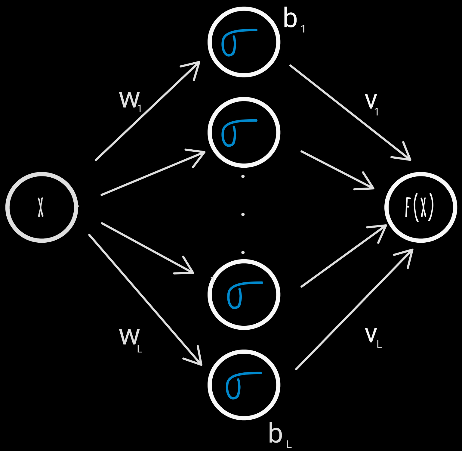 |
We have $\color{white}{\mathsf{L}}$ nodes, with sigmoid activation, each parametrized with weight $\color{white}{\mathsf{w_k}}$ and bias $\color{white}{\mathsf{b_k}}$, while the output layer is linear, with weight $\color{white}{\mathsf{v_k}}$ for each incoming result from the hidden layer |
So how do we find the parameters $\mathsf{w_k}$, $\mathsf{b_k}$, and $\mathsf{v_k}$?
The Loss Function
If I had a genie that could grant we any wish, I would ask him - please provide me the set of values for $\mathsf{w_k}$, $\mathsf{b_k}$, and $\mathsf{v_k}$, for which our bespoke function $\mathsf{f(x)}$ is as close as possible to the unknown target function $\mathsf{y}$.
In other words, dear genie, please minimize the distance between $\mathsf{f(x)}$ and $\mathsf{y}$, for all the $n$ observed points of $\mathsf{y}$. The genie smiles and gives me the following function:
| $\mathsf{ C(w, b, v) = \dfrac{1} {2n} \displaystyle\sum\limits_{i = 1}^{n} (f({x_i}) - {y_i})^2 }$ |
| This is known as the loss function, and our ideal parameter values should minimize this. For $n$ samples of the target function, we want our approximated function to minimize the error, i.e. get as close as possible to the given target values. We only want the distance between the two functions, we don't care if the difference between them is $1$ or $-1$, which is where taking the square of their difference helps. We divide by $n$ to remove dependence of the error on the size of $n$. Why did we divide by $2$ as well? The genie said "It will be kind of convenient when you take the derivative bro". I don't know what that means |
Now that we have formulated our wish into a function, we can proceed to minimize it and get our desired parameters. Note that this isn't the only possible loss function, you can get different ones, by asking more specific wishes to the genie.
Gradient Descent
To find best set of parameter values that minimize $\mathsf{ C(w, b, v) }$, we just need to iterate through all possible values of $\mathsf{w_k}$, $\mathsf{b_k}$, and $\mathsf{v_k}$, and see where the loss function is lowest! The only problem is, our parameters are real numbers, and their possible values lie in the range $(-\infty , \infty )$.
For now, let's assign some random values to our parameters, and evaluate $\mathsf{ C(w, b, v) }$. If we're lucky these initial values might be the optimal ones. Possible, but very, very unlikely. We may not get the optimal result in a single shot, but what if we could move toward it, one step at a time?
The idea is simple - keep moving towards the direction $\mathsf{ C(w, b, v) }$ is decreasing, by using its gradient. If we carefully keep take our steps, we will eventually reach the minimum. Or, to put it simply:
| $\mathsf{ w \longrightarrow w - \eta\dfrac{\partial C}{\partial w} }$ | $\mathsf{ b \longrightarrow b - \eta\dfrac{\partial C}{\partial b} }$ | $\mathsf{ v \longrightarrow v - \eta\dfrac{\partial C}{\partial v} }$ |
| We iteratively update our parameters by subtracting the gradient of $\mathsf{ C(w, b, v) }$ with respect to them (hence partial derivatives). $\mathsf{\eta}$ is a constant that determines the speed of our optimization, i.e. how carefully we are taking our steps. If it's too high, we might overstep and miss the minimum, but if it's too low, we might take a lot more time than necessary to reach our goal. $\mathsf{\eta}$ is called the learning rate, and is an example of a hyper-parameter, and we set its value based on heuristics, gut feelings, and astrology. | ||
A quick note before we proceed - the derivative of the sigmoid is given by:
| $\mathsf{\dfrac{d\sigma(\mathit{x})}{d\mathit{x}} = \sigma(\mathit{x})(1 - \sigma(\mathit{x})) }$ |
Now we just need to find $\mathsf{ \dfrac{\partial C}{\partial w} }$, $\mathsf{ \dfrac{\partial C}{\partial b} }$, and $\mathsf{ \dfrac{\partial C}{\partial v} }$. Which requires application of the chain rule, and use of the sigmoid derivative formula we mentioned above. To put it simply:
| $\mathsf{\dfrac{\partial C }{\partial {w_k} } = \dfrac{1} {n} \displaystyle\sum\limits_{i = 1}^n (f(x_i) - y_i) \dfrac{\partial f(x_i) }{\partial{w_k} } \\ = \dfrac{1} {n} \displaystyle\sum\limits_{i = 1}^n (f(x_i) - y_i) {v_k} \dfrac{\partial \sigma( {w_k} {x_i} + {b_k} ) }{\partial {w_k} } \\ = \dfrac{v_k} {n} \displaystyle\sum\limits_{i = 1}^n (f(x_i) - y_i) \sigma( {w_k} {x_i} + {b_k} ) (1 - \sigma( {w_k} {x_i} + {b_k} )) x_i }$ |
| $\mathsf{ \dfrac{\partial C }{\partial{b_k} } = \dfrac{v_k} {n} \displaystyle\sum\limits_{i = 1}^n (f(x_i) - y_i) \sigma( {w_k} {x_i} + {b_k} ) (1 - \sigma( {w_k} {x_i} + {b_k} )) }$ |
| $\mathsf{ \dfrac{\partial C }{\partial{v_k} } = \dfrac{1} {n} \displaystyle\sum\limits_{i = 1}^n (f(x_i) - y_i) \sigma( {w_k} {x_i} + {b_k} ) }$ |
The Algorithm
- Choose some value for $\mathsf{L}$ - the number of nodes in the hidden layer. A large value might get a better fit, but will be slower and more computationally intensive, whereas a value too small may not lead to good fit.
- Choose some value for $\mathsf{\eta}$ - a good value for $\mathsf{\eta}$ has to be determined experimentally.
- Initialize the parameters to random values.
- For a fixed number of iterations, update the values of all the parameters by gradient descent.
- Profit.
Fun
Enough talk! Enough maths! Here are some animations -
| $\mathsf{L = 5, \eta = 0.05}$ |
|---|
It’s trying, but clearly, 5 nodes are not enough. More nodes!
| $\mathsf{L = 25, \eta = 0.05}$ |
|---|
A lot more satisfying! But the fit isn’t good enough towards the right. Let’s increase $\mathsf{L}$ slightly more.
| $\mathsf{L = 30, \eta = 0.05}$ |
|---|
That hits the spot! Look at it! Perfect. This is way better than Netflix.
We can try increasing $\mathsf{L}$ further but be careful - the curve might gain sentience and take over the planet.
To cap it off here is our neural net trying to fit over some other functions.
| $\mathsf{L = 30, \eta = 0.05}$ | $\mathsf{L = 30, \eta = 0.05}$ |
|---|---|
| $\mathsf{L = 30, \eta = 0.05}$ | $\mathsf{L = 50, \eta = 0.05}$ |
Here’s the notebook where you can play with different functions.